As ACCS is completely integrated within ANSYS Workbench, one simply needs to run Workbench to have access to it. For step-by-step tutorials, please refer to the Workshops section.
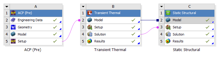
A typical Workbench ACCS workflow for composite structures looks as follows:
Fig. 1.1.1 Typical cure simulation workflow for composites in Workbench.
The material properties are defined in the Engineering Data module. A shell model is generated in DesignModeler or in SpaceClaim or in any other CAD tool, then it is worked out in ACP (Pre) module to build a solid finite element model of the composite structure that will be transferred to the “Transient Thermal” module where the temperature distribution will be computed throughout the cure cycle for every element as well as the degree of cure, the state of the material, the glass transition temperature and the instantaneous heat of reaction. The temperature distribution is then transferred to the “Static Structural” module where the distortions will be computed using the previously computed temperature and the material properties.
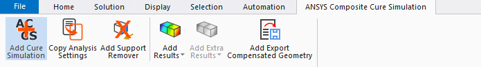
The ACCS solution is also integrated within Mechanical and is therefore available in the Transient Thermal and Static Structural analysis systems in the form of an additional tab in the ribbon as show in the figure below.
Fig. 1.2.3 ACCS features in the Mechanical menu ribbon.
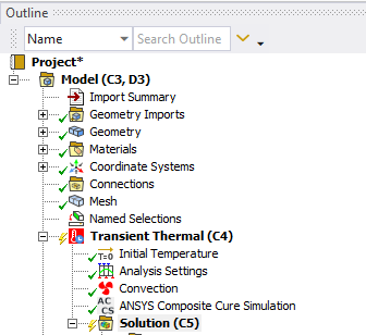
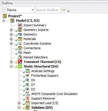
Adding ACCS to the analysis invokes the ANSYS solver with chemical cure and cure shrinkage routines for materials with defined cure kinetics properties within the Engineering Data module. Once in Workbench Mechanical the user can initiate ACCS by clicking on the “Add Cure Simulation” button as shown in the figures below for the Transient Thermal and Static Structural modules.
Fig. 1.2.4 Initiating ACCS from the toolbar adds an “ANSYS Composite Cure Simulation” item to the current thermal analysis.
Fig. 1.2.5 Initiating ACCS from the toolbar adds an “ANSYS Composite Cure Simulation” item to the current structural analysis.
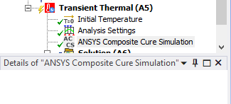
Fig. 1.2.6 Details of the options for “ANSYS Composite Cure Simulation” item for a thermal analysis.
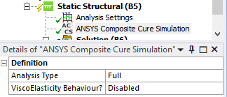
Fig. 1.2.7 Details of the options for “ANSYS Composite Cure Simulation” item for a FULL structural analysis.
The “ViscoElasticity Behaviour?” dropdown menu allows to enable/disable viscoelasticity without the need to modify the materials in Engineering Data.
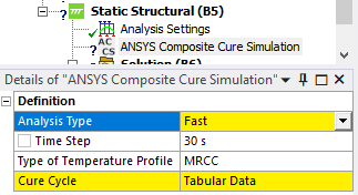
Fig. 1.2.8 Details of the options for “ANSYS Composite Cure Simulation” item for a FAST structural analysis.
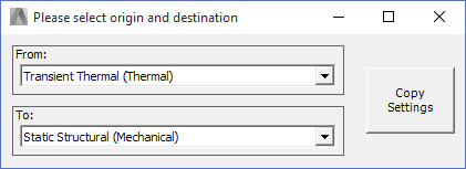
When performing a Full Cure Simulation, the button “Copy Analysis Settings” allows the user to copy relevant analysis settings between two analyses easy and fast.
Fig. 1.3.6 This pop up window appears when selecting the “copy Analysis Settings” feature.
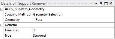
The lamination process usually involves the placing of composite layers over a mold. After the curing cycle is finished, the part is taken off the mold. Is in this phase of the process where the most relevant permanent deformations occur since the part is without the form constrictions. To simulate that step, ACCS has a boundary condition called “Support Remover” which delete every node that is scoped to it from it predefined displacement constraint. It is important to remark that the support remover is only needed for frictionless supports because you cannot enable/disable it per load step as other supports do.
Fig. 1.4.6 Details of the Support Remover options
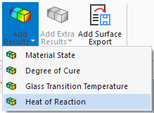
Including the ACCS feature into the analysis opens the possibility to add cure simulation specific post-processing options like Material State, Degree of Cure, Glass Transition Temperature and Cure Shrinkage in all cartesian directions. These options can be found by selecting the “Add Results” and the “Add Extra Results” buttons, as shown in the following image:
Fig. 1.5.1 Results available during both the Thermal and Mechanical analyses.
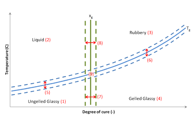
There are two main transitions that can be distinguished during the curing process of a thermosetting resin. The first one is gelation and the second one is vitrification occurring when the material Tg reaches the cure temperature
Fig. 1.5.2 Plot of an empirical curve (blue) and a simplified curve (red dots) used by ACCS to describe the different material states.
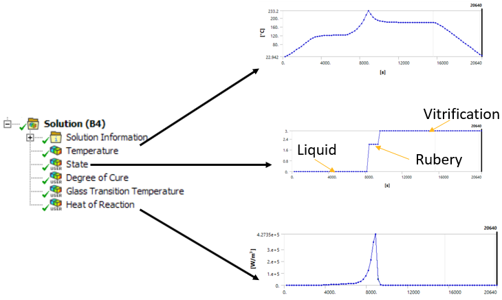
This result shows the develope of the curing reaction in the material domain. See Fig. 3.1.1 to see a the dependence of the degree of cure and the temperature in time.
The Heat of Reaction is shown in the Thermoset domain and the plot shows the evolution of it in the time window.
Once the model is solved, the results can be reviewed by clicking on them. Here in the example, an exothermic reaction can be seen in the temperature profile. In many cases, the exothermic reaction a risk to the process. Excessive heat can cause inhomogeneous cure (check the Degree of Cure result) and can damage the structural materials (mainly the resin itself, but also polymeric sandwich cores; or heat-sensitive fibers, such as natural fibers), as well as the auxiliary materials (e.g. the vacuum bag).
Fig. 1.5.3 Solution plots example. Exotherms and material states can be post processed from thermal simulation.
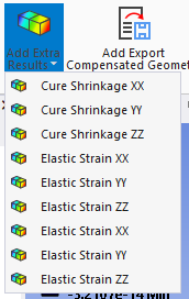
Fig. 1.5.4 Extra results only available during the Mechanical analysis.
Warning
Strain Results: It is important to note that the normal and shear strain results in mechanical do not only contain the elastic strains but also the cure shrinkage. To view on the elastic strains, please add the “Elastic Strain” results available in the “Extra Results” menu.
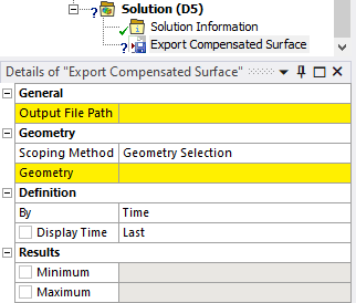
The export compensated geometry button adds an object which automatically compensates the process induced distortions for the selected faces. The process induced distortions (deformations) of the structural simulation are inverted and added to the nominal geometry. The compensated geometry can be exported as STL, RSO or point cloud. The options of the support remover are:
Output File Path: the file path where the file will be saved
Scoping Method and Geometry: the geometrical entities which will be exported
Fig. 1.6.1 Options of the compensated surface export item.
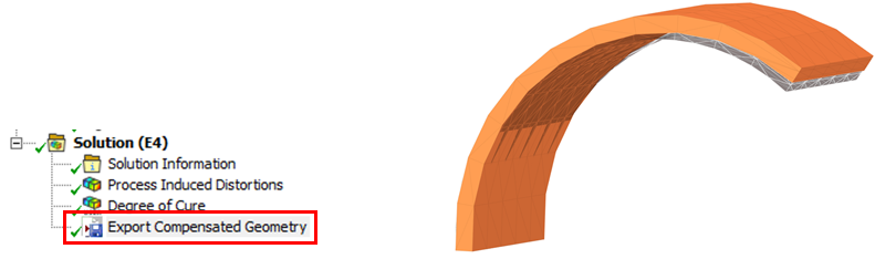
Fig. 1.6.2 Compensated geometry (orange) and nominal shape (grey).
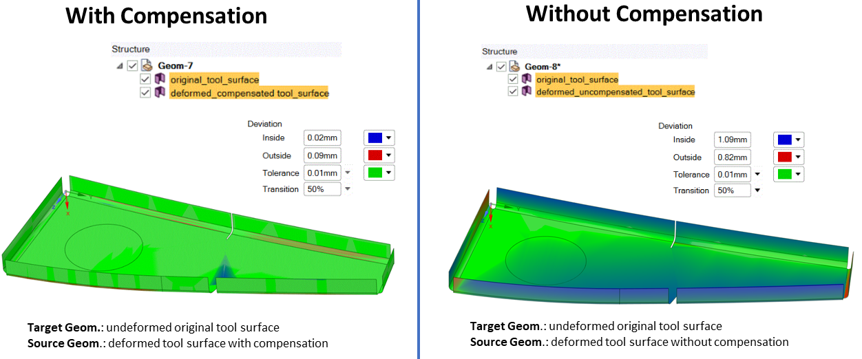
The compensated STL geometry can be natively imported into SpaceClaim to morph the starting mold geometry and realize a tool compensation with a Class A finish, further details and a complete example is given in the ACCS tutorial on the ALH.
ACCS does not support Ansys RSM (Remote Solve Manager).
ACCS does not support coupled simulations in Ansys Mechanical, the transient thermal analysis to predict the evolution of degree of curing and thermal behavior during processing is independent of the downstream structural simulation and, therefore, the two simulations are sequentially coupled.
The viscoelasticity (Prony) implementation is currently implemented only for small-deformation studies.
 adds an object which automatically compensates the process induced distortions for the selected faces. The process induced distortions (deformations) of the structural simulation are inverted and added to the nominal geometry. The compensated geometry can be exported as STL, RSO or point cloud. The options of the support remover are: