1. Usage Reference

As ACCS is completely integrated within ANSYS Workbench, one simply needs to run Workbench to have access to it. For step-by-step tutorials, please refer to the Workshops section.

1.1. ACCS RTM Solver Workflow

A typical Workbench ACCS RTM Solver workflow for composite structures looks as follows:

1.1.1. Typical Workflow With ACP

The material properties are defined in the Engineering Data module. A shell model is generated in DesignModeler or in SpaceClaim or in any other CAD tool, then it is worked out in ACP (Pre) module to build a solid finite element model of the composite structure that will be transferred to the “RTM Solver” module where the flow will be calculated.

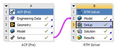
Fig. 1.1.2 Typical ACCS RTM Solver workflow for composites in Workbench.

1.1.2. Workflow With Only ACCS RTM Solver

For workflows with only an ACCS RTM Solver, an external engineering data module is required to be created, and then imported into the model.

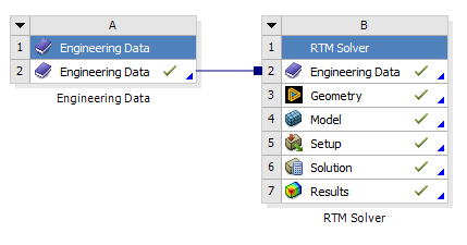
Fig. 1.1.3 ACCS RTM Solver workflow with only the solver.

1.1.3. Workflow With External Model and ACP

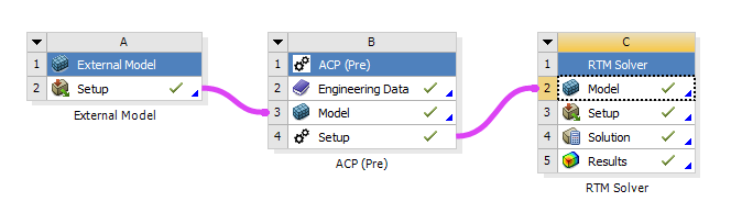
Fig. 1.1.4 ACCS RTM Solver workflow with External Model and ACP.

1.2. ACCS RTM Solver Material Definitions

There are two types of materials needing to be defined in ACCS RTM Solver. These are fabrics and resins. This section will detail the compulsory properties for each of these material types, as well as optional ones.

1.2.1. Fabric Material Definition

For fabrics, only permeability needs to be specified. However, note that in solver versions 25R2 and earlier, porosity is assumed to be constant throughout the model. In later versions, porosity can be defined. To properly account for porosity in simulations:

• When using pressure inlets: Divide the fabric’s permeability by the porosity.

• When using flow rate inlets: Divide the flow rate by the model’s average porosity.

Note

The solver provides equivalent pressure values when defining flow rate inlets this way. To obtain the actual pressure, multiply the output pressure by the average porosity.

It is important to note that in solver versions 25R2 and earlier, mixed inlet definitions are not supported if porosity needs to be factored into the fabric material properties.

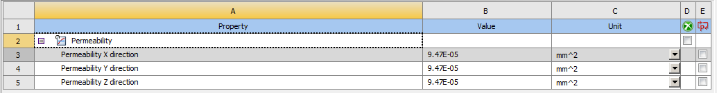
Fig. 1.2.9 An example definition of a fabric material in ACCS RTM Solver.

1.2.2. Resin Material Definition

For resins, only viscosity is required to be defined. However, if gravitational effects are to be simulated, density will need to be set.

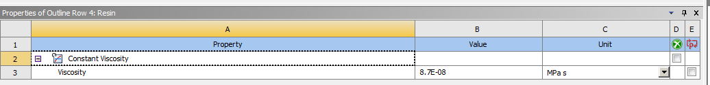
Fig. 1.2.10 An example definition of a resin material in ACCS RTM Solver.

If the gelation properties of a material are set, a cure kinetic equation and cure defined viscosity are required to be defined. The ACCS RTM Solver currently supports Nth Order, Autocatalytic and Kamal-Sourour cure kinetic equations.

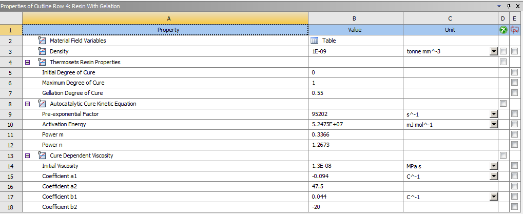
Fig. 1.2.11 An example definition of a resin material in ACCS RTM Solver with gelation properties and density set.

Note

For workflows containing only ACCS RTM Solver, engineering data will need to be defined in an external engineering data module, then imported into the solver.

1.3. ACCS RTM Solver Boundary Conditions

There are three main types of boundary conditions in ACCS RTM Solver: inlets, outlets and thermal conditions. Inlets and outlets are required boundary conditions for the simulation to run, while thermal conditions are required only if temperature dependent viscosity is desired. Any other type of Ansys Mechanical boundary conditions will be ignored.

1.3.1. Inlets

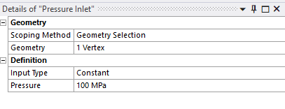
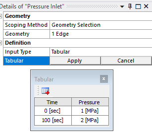
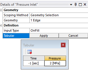
Inlets can be defined based on either pressure or flow rate. Additionally, time-dependent inlets can be configured to open at a specific time or when the resin reaches a designated node. Inlet selection can be selected using Ansys geometry selection tools or named selections. There are three input types available to you when defining inlets: “Constant”, “Tabular” and “OnFill”.

Input Type	Description	Image
Constant	The pressure or flow rate remains static throughout the simulation.
Tabular	The pressure or flow rate can be defined at different time points, with values interpolated between defined time points based on the given data.
OnFill	The inlet opens when the resin reaches it. “-1” indicates OnFill.

Warning

When a flow rate inlet is defined, the specified flow rate is applied to each selected node within the geometry. If your intent is to apply the total flow rate across the entire selected geometry (rather than per node), you must divide the total flow rate by the number of selected nodes.

1.3.2. Outlets

Outlets are exit points where the resin flows out of the model. The simulation terminates once all nodes associated with an outlet are fully filled. Outlets can be selected using Ansys geometry selection tools or named selections.

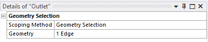
Fig. 1.3.7 ACCS RTM Solver outlet definition.

1.3.3. Thermal Conditions

Thermal conditions from Ansys Mechanical can be used to define the temperature profile for the simulation, typically to establish the curing cycle during the infusion process.

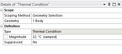
Fig. 1.3.8 ACCS RTM Solver thermal condition definition.

1.3.4. Thermal Import

Temperature profiles from transient thermal simulations can be imported by selecting the corresponding result file within a Thermal Import load. If only one transient thermal result is available in the project, it will be automatically selected. The imported temperature data is then applied to the selected geometry in the ACCS RTM Solver model. The geometry can be selected using selected using Ansys geometry selection tools or named selections.

Warning

Temperature values from thermal imports will take priority over other definitions.

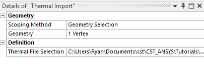
Fig. 1.3.9 ACCS RTM Solver thermal import definition.

1.3.5. Environment Temperature

Environment temperature is defined as normal. For parts of the model with no temperature definition, the environment temperature will be used.

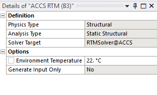
Fig. 1.3.10 Environment Temperature definition.

1.4. ACCS RTM Solver Analysis Settings

Within “Analysis Settings”, you will find additional options to further define your infusion model.

Parameter	Description
Result Only	If result import is defined in the tree, this option should be defined as “True”. Otherwise, it should be “False”.
Result Step Increment	This parameter defines the frequency at which the solver writes results to the output file. A value of N specifies that the solver will record data every N steps. For example, setting this parameter to 10 ensures that output is written only once every 10 steps, reducing file write frequency and decreasing final output file size.
Number Of Cores Used	This parameter defines the number of virtual cores used by the solver. If the value is larger than the number of cores on the machine M, it will use M cores.
Air Entrapment Pressure	This parameter defines the initial pressure for each entrapment that occurs during the simulation. The pressure for the entrapment is then updated at every increment, based on the changing volume of the entrapment. If entrapment is set to zero, no entrapment calculations will be made.
Overfill Factor	The overfill factor scales the step time increment. It is calculated as: \(\text{Time Step Increment} = \text{Overfill Factor} \times \text{Step Time Increment}\) By default, the overfill factor is set to 1, meaning the step time increment corresponds to the time required for another node to be filled. Adjusting this factor allows you to control the speed at which the simulation progresses, affecting the time taken to fill the resin during the infusion process. While this may make the simulation run faster, it may impact the accuracy of the result.
Minimum Pressure	Defines the minimum pressure allowed for the inlets during the simulation. The inlets are checked on each iteration, and if the pressure falls below the set value, the simulation will terminate. If set to 0, no limit is placed.
Maximum Pressure	Defines the maximum pressure allowed for the inlets during the simulation. The inlets are checked on each iteration, and if the pressure exceeds the set value, the simulation will terminate. If set to 0, no limit is placed.
Minimum Flow	Defines the minimum flow rate allowed for the inlets during the simulation. The inlets are checked on each iteration, and if the flow rate falls below the set value, the simulation will terminate. If set to 0, no limit is placed.
Maximum Flow	Defines the maximum flow rate allowed for the inlets during the simulation. The inlets are checked on each iteration, and if the flow rate exceeds the set value, the simulation will terminate. If set to 0, no limit is placed.
Gravitational Constant X	This parameter determines the X component of the gravitational vector. The value is applied directly to the resin’s X direction flow rate.
Gravitational Constant Y	This parameter determines the Y component of the gravitational vector. The value is applied directly to the resin’s Y direction flow rate.
Gravitational Constant Z	This parameter determines the Z component of the gravitational vector. The value is applied directly to the resin’s Z direction flow rate.
Maximum Infusion Time	This parameter controls the infusion time at which the solver will terminate. If it is set to 0, the solver will run until all outlets are filled or until any other limits are reached. If no limits are reached, the solver will need to be manually terminated.
Resin Material	This setting controls the resin used in the infusion model.
Thermal Mechanical Results	This setting enables or disables the calculation of thermal mechanical results.

1.5. ACCS RTM Solver Post-Processing Options

Several results can be added to the model, allowing for simulation specific post-processing options like Fill, Infusion Time, and Flow Rate. These options can be found by selecting the “Main Results” and the “Other Results” buttons, as shown in the following image:

1.5.1. Main Results

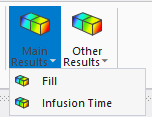
Fig. 1.5.5 Results available during ACCS RTM Solver analysis.

Result Type	Description
Fill	This result shows the fill of each node, as the simulation progresses. Fill is defined as the percentage of nodal volume filled by resin. IE: 0.3 would mean that 30% of the node is filled with resin. This result is typically used to visualise the flow front.
Infusion Time	This result shows for each node, the time at which it was fully filled.

1.5.2. Other Results

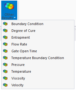
Fig. 1.5.6 Extra results available in the “Other Results” tab.

Result Type	Description
Degree of Cure	This result shows the degree of cure for each node. IE: 0.3 would be 30% degree of cure. Warning This result only displays values when gelation is set for the resin material.
Entrapment	This result shows the entrapment pressure in the model for each node, if entrapment is set.
Flow Rate	This result shows, for each node, the volume of resin flowing in and out per second. This is valuable for assessing the risk of resin pooling within a component, as areas with high flow rates are more prone to resin accumulation.
Gate Open Time	This result shows for each node, the open time of the source inlet that filled the node.
Pressure	This result shows the pressure values at each node.
Boundary Conditions	This result shows the pressures of the statically defined inlets and outlets. Note Even if a flow rate inlet is set, this will show only pressure.
Temporal Boundary Conditions	This result shows the pressure for nodes where time dependent boundary inlets are set.
Velocity	This result shows the resin flow velocity at each node.
Viscosity	This result shows the viscosity values at each node.
Tg	This result shows the glass transition temperature values at each node.
Resin State	This result shows the Resin State of each node: 0 = No Resin, 1 = Liquid, 2 = Rubbery, 3 = Glassy.
Thermal Expansion	This result shows the strain from thermal expansion at each node (calculated from volume change due to thermal expansion).
Cure Shrinkage	This result shows the strain from cure shrinkage at each node (calculated from volume change due to cure shrinkage).
Total Volume Change	This result shows the Total Volume Change at each node.

Once the model is solved, the results can be reviewed by clicking on them. Here in the example we can see the fill at 12.5 seconds in the model.

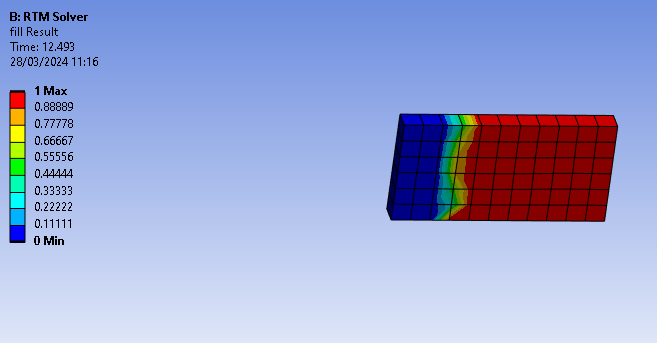
Fig. 1.5.7 Solution plots example. Fill of each node at 25 seconds

Warning

It is important to note that the above results will only work with the ACCS RTM Solver.

1.6. ACCS RTM Solver Importing Results

1. Ensure that the mesh in mechanical is identicial to that of the result.

2. Select “Import Result” in the ACCS RTM Solver ribbon to add a import result load. Click on the load, and select the H5 file you wish to import from.

3. Set the analysis setting “Result Only” to True.

4. Choose the results you want to view from the ACCS RTM Solver ribbon.

5. Press solve.

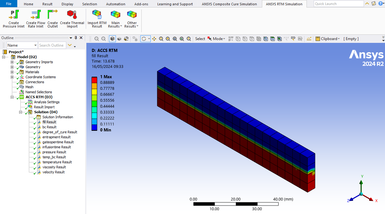
Fig. 1.6.4 Example of an imported result.

1.7. Using command line to run ACCS RTM Solver

1. Setup your model in Ansys as normal.

2. In Ansys Mechanical select “Write Input File” in the Solution ribbon to write the input files (the solution tree object needs to be selected to see this tab).

3. Run the RTM Solver by command line with > %ProgramFiles%\LMAT\ACCS\v3.2hf1_WB25.2\RTM\Resin_Infusion.exe <RTWFilePath> where <RTWFilePath> is the filepath of the RTW file for the model.

4. Import the H5 result back into Ansys to view the result.

Fig. 1.7.1 Write Input File button.

1.8. Known Limitations

1. The graph from the results will only show the first second. However the animation and tabular data will display as normal.

2. ACCS properties will not be shown in the Engineering Data section of the ACCS RTM Solver module. Please use an external Engineering Data and import it in, or define the material property in ACP if you are defining layups.

3. ACCS RTM Solver only supports ACP defined layups.